Denoising Multi-Channel Images
Auto-Denoise (autoden) provides implementations for a variety of unsupervised and self-supervised Convolutional Neural Network (CNN) denoising methods. This tutorial will guide you through setting up the data, training different denoisers, performing inference, and visualizing the results for multi-channel images.
Setting Up the Data
First, we need to set up the data to be used for training and testing the denoisers. We will use the skimage library to generate a noisy image and create multiple noisy versions of it.
import matplotlib.pyplot as plt
import numpy as np
import skimage.data as skd
import skimage.transform as skt
from copy import deepcopy
from numpy.typing import NDArray
from tqdm.auto import tqdm
import autoden as ad

%load_ext autoreload
%autoreload 2

%matplotlib widget

USE_CAMERA_MAN = True
NUM_IMGS_TRN = 4
NUM_IMGS_TST = 2
NUM_IMGS_TOT = NUM_IMGS_TRN + NUM_IMGS_TST

EPOCHS = 1024
REG_TV_VAL = 1e-7

img_orig = skd.cat().astype(np.float32)
img_orig = skt.downscale_local_mean(img_orig, (4, 4, 1))
print(img_orig.shape)
img_orig *= 255 / img_orig.max()

imgs_noisy: NDArray = np.stack(
    [(img_orig + 20 * np.random.randn(*img_orig.shape)) for _ in tqdm(range(NUM_IMGS_TOT), desc="Create noisy images")],
    axis=0,
)

print(f"Img orig -> [{img_orig.min()}, {img_orig.max()}], Img noisy -> [{imgs_noisy[0].min()}, {imgs_noisy[0].max()}]")
print(f"Img shape: {img_orig.shape}")
Training vs testing images
Certain algorithms require to allocate a certain number of input images to the test set.
This set is used to verify the model's training convergence, and to select the most appropriate epoch.
The variable tst_inds serves this purpose, by containing the indexes of the images to use for testing.
The algorithms that do not use this variable, will randomly select a certain fixed number of pixels as leave-out set.
Training the Denoisers
We will train four different denoisers: Supervised Denoiser, Noise2Noise (N2N), Noise2Void (N2V), and Deep Image Prior (DIP). We first define the type of model that we will want to use. In this case it will be a U-net [1], with 16 features:
net_params = ad.NetworkParamsUNet(n_channels_in=3, n_channels_out=3, n_features=16)
The variable net_params only defines the type of architecture that we want. When passed to the denoising algorithms, they will use it to create and initialize a U-net model.
Other pre-configured models are available: MS-D net [2], DnCNN [3], and a custom ResNet implementation [4].
Compared to single-channel image denoising, here, we need to specify the n_channels_in and n_channels_out arguments to be equal to the number of input and target channels, respectively. Since we are dealing with RGB images, it will be 3 for both.
Working with complex signals
When working on complex signals, the prepare_data method will convert them into real signals, by splitting the real and imaginary parts to two different channels. This means that if you had a single-channel signal, it will be processed as two-channel. If you already had a multi-channel signal, the real and imaginary parts of the channels will be concatenated.
1D and 3D signals
We have recently introduced the support for 1D and 3D signals in auto-denoise.
To correctly process these signals, it is enough to instantiate a model with the correct dimensionality.
This means that we need to set the correct value for the parameter n_dims in the model definition:
net_params = ad.NetworkParamsUNet(n_channels_in=3, n_channels_out=3, n_features=16, n_dims=1) # 1D Convolutions
net_params = ad.NetworkParamsUNet(n_channels_in=3, n_channels_out=3, n_features=16, n_dims=3) # 3D Convolutions
Using a 2D model with 3D data
It is possible to use a 3D dataset with a 2D model. The depth direction will be interpreted as the batch dimension. The 2D model will interpret each volume slice as a different image example.
This could be useful in GPU memory constrained scenarios, where the higher memory requirements of 3D convolutions (w.r.t. 2D convolutions) could exceed the available GPU memory. This technique could save around 30\% memory, but it would lose the information along the depth direction.
This will not impact the correct handling of multi-channel signals. The user should just remember that the channels will be reordered, and the channel axis will end up in between the depth axis and the other two (height and width).
Supervised Denoiser
The supervised denoiser is trained using pairs of noisy and clean images. It learns to map noisy images to their clean counterparts.
denoiser_sup = ad.Supervised(model=deepcopy(model), reg_val=REG_TV_VAL)
sup_data = denoiser_sup.prepare_data(imgs_noisy, img_orig, num_tst_ratio=NUM_IMGS_TST / NUM_IMGS_TOT, channel_axis=-1)
denoiser_sup.train(*sup_data, epochs=EPOCHS)
Here, we know that scikit-image puts the RGB axis as last, so we specify that to the prepare_data method, through the parameter channel_axis. The data will automatically be reordered to be in the expected layout by PyTorch's convolutions.
Noise2Void (N2V)
Noise2Void is a self-supervised denoising method that can work with a single noisy image [5]. This implementation can also work with structured noise [6]. It applies randomly generated masks to the images and learns to predict the masked pixels.
denoiser_n2v = ad.N2V(model=deepcopy(model), reg_val=REG_TV_VAL)
n2v_data = denoiser_sup.prepare_data(imgs_noisy, img_orig, num_tst_ratio=NUM_IMGS_TST / NUM_IMGS_TOT, channel_axis=-1)
denoiser_n2v.train(*n2v_data, epochs=EPOCHS)
As for the Supervised algorithm, we use the parameter channel_axis to specify which is the RGB axis.
Noise2Noise (N2N)
Noise2Noise is a self-supervised denoising method that uses pairs of noisy images of the same object [7]. It learns to map one noisy image to another noisy image of the same object. The prepare_data function is used to organize the data in such a way that the algorithm can handle it correctly.
denoiser_n2n = ad.N2N(model=deepcopy(model), reg_val=REG_TV_VAL)
n2n_data = denoiser_n2n.prepare_data(imgs_noisy, channel_axis=-1)
denoiser_n2n.train(*n2n_data, epochs=EPOCHS)
As for the Supervised and Noise2Void algorithms, we use the parameter channel_axis to specify which is the RGB axis.
Batched processing
N2N and Supervised support batched processing (both during training and inference). This is usually required for large datasets, where they cannot fully fit into GPU memory.
The batch size is selected through the batch_size argument when N2N is initialized.
denoiser_sup = ad.Supervised(model=net_params, reg_val=REG_TV_VAL, batch_size=16)
and
denoiser_n2n = ad.N2N(model=net_params, reg_val=REG_TV_VAL, batch_size=16)
Data augmentation
N2N and Supervised also support data augmentation in the form of image and volume flips. This could be used to virtually increase the data size during training.
denoiser_sup = ad.Supervised(model=net_params, reg_val=REG_TV_VAL, augmentation="flip")
and
denoiser_n2n = ad.N2N(model=net_params, reg_val=REG_TV_VAL, augmentation="flip")
Deep Image Prior (DIP)
Deep Image Prior is an unsupervised denoising method that can also work with a single image [8]. It uses the prior knowledge embedded in the network architecture to denoise the image. The prepare_data function is used to organize the data in such a way that the algorithm can handle it correctly.
denoiser_dip = ad.DIP(model=deepcopy(model), reg_val=REG_TV_VAL * 2.5e1)
dip_data = denoiser_dip.prepare_data(imgs_noisy, channel_axis=-1)
denoiser_dip.train(*dip_data, epochs=EPOCHS * 3)
As for the other algorithms, we use the parameter channel_axis to specify which is the RGB axis.
Regularization weight
The DIP is more sensitive to the regularization weight, and it can be adjusted to obtain better results.
Performing Inference
Inference is the process of using the trained models to denoise new images. The infer method takes the noisy images as input and outputs the denoised images. The infer method takes a channel_axis_dst argument that allows us to output data in the same format as it was passed to prepare_data, i.e., move back the multi-channel axis to its original position.
Inference input
The output of the prepare_data function is needed for inference.
Supervised Denoiser Inference
den_sup = denoiser_sup.infer(sup_data[0], channel_axis_dst=-1).mean(0)
Inference input
The output of the prepare_data function is preferred for the inference of Supervised, even though the noisy images should also work for the foreseeable future, provided that the axes are correctly organized.
Noise2Void (N2V) Inference
den_n2v = denoiser_n2v.infer(n2v_data[0], channel_axis_dst=-1).mean(0)
Inference input
The output of the prepare_data function is preferred for the inference of Noise2Noise, even though the noisy images should also work for the foreseeable future, provided that the axes are correctly organized.
Noise2Noise (N2N) Inference
den_n2n = denoiser_n2n.infer(n2n_data[0], channel_axis_dst=-1)
Inference output
The inference function of N2N automatically averages the splits, unless the average_splits flag is set to False.
Deep Image Prior (DIP) Inference
den_dip = denoiser_dip.infer(dip_data[0], channel_axis_dst=-1)
Inference input
The output of the prepare_data function is also needed for the inference of DIP.
Visualizing the Results
Finally, we visualize the results of the different denoisers.
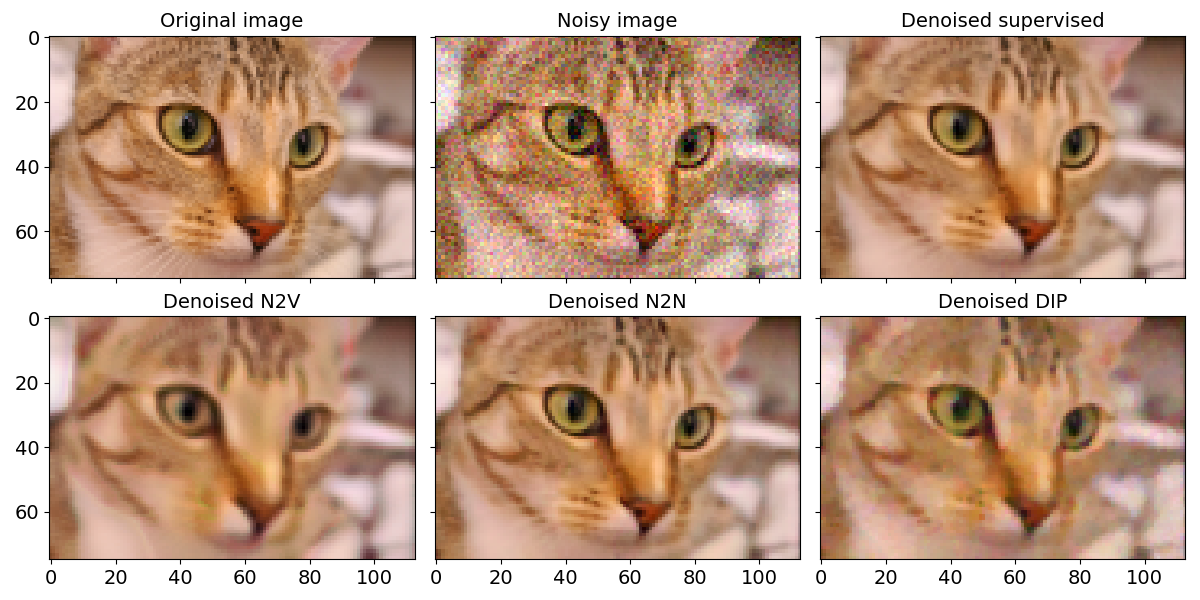
fontsize = 14

fig, axs = plt.subplots(2, 3, sharex=True, sharey=True, figsize=(12, 6))
axs[0, 0].imshow(img_orig / 255)
axs[0, 0].set_title("Original image", fontsize=fontsize)
axs[0, 1].imshow(imgs_noisy[0] / 255)
axs[0, 1].set_title("Noisy image", fontsize=fontsize)
axs[0, 2].imshow(den_sup / 255)
axs[0, 2].set_title("Denoised supervised", fontsize=fontsize)
axs[1, 0].imshow(den_n2v / 255)
axs[1, 0].set_title("Denoised N2V", fontsize=fontsize)
axs[1, 1].imshow(den_n2n / 255)
axs[1, 1].set_title("Denoised N2N", fontsize=fontsize)
axs[1, 2].imshow(den_dip / 255)
axs[1, 2].set_title("Denoised DIP", fontsize=fontsize)
for ax in axs.flatten():
    ax.tick_params(labelsize=fontsize)
fig.tight_layout()
plt.show(block=False)
And here below we present the PSNR (Peak Signal-to-Noise Ration), SSIM (Structural Similarity Index) and FRC (Fourier Ring Correlation) of the results.
PSNR:
- Supervised: 33.7
- Noise2Void: 26.1
- Noise2Noise: 32.6
- Deep Image Prior: 29.7
SSIM:
- Supervised: 0.901
- Noise2Void: 0.776
- Noise2Noise: 0.884
- Deep Image Prior: 0.825
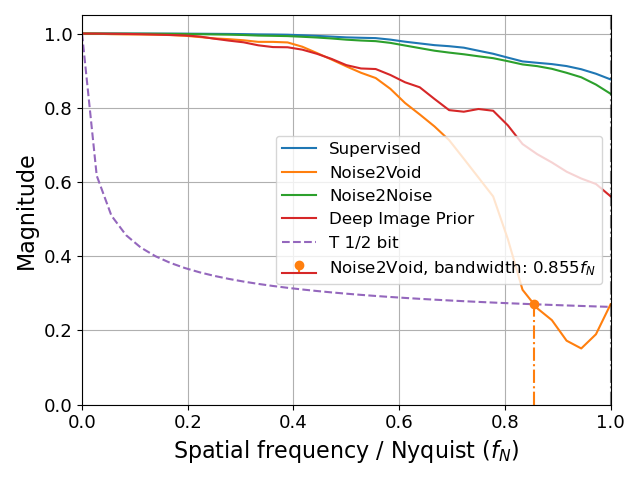
from corrct.processing.post import plot_frcs
from skimage.metrics import peak_signal_noise_ratio as psnr
from skimage.metrics import structural_similarity as ssim

all_recs = [den_sup, den_n2v, den_n2n, den_dip]
all_labs = ["Supervised", "Noise2Void", "Noise2Noise", "Deep Image Prior"]

data_range = img_orig.max() - img_orig.min()
print("PSNR:")
for rec, lab in zip(all_recs, all_labs):
    print(f"- {lab}: {psnr(img_orig, rec, data_range=data_range):.3}")
print("SSIM:")
for rec, lab in zip(all_recs, all_labs):
    print(f"- {lab}: {ssim(img_orig, rec, data_range=data_range, channel_axis=-1):.3}")

plot_frcs([(img_orig.astype(np.float32), rec) for rec in all_recs], all_labs, axes=(-3, -2))
References
- O. Ronneberger, P. Fischer, and T. Brox, “U-Net: Convolutional Networks for Biomedical Image Segmentation,” in Medical Image Computing and Computer-Assisted Intervention – MICCAI 2015, 2015, pp. 234–241. doi: 10.1007/978-3-319-24574-4_28.
- D. M. Pelt and J. A. Sethian, “A mixed-scale dense convolutional neural network for image analysis,” Proceedings of the National Academy of Sciences, vol. 115, no. 2, pp. 254–259, 2018, doi: 10.1073/pnas.1715832114.
- K. Zhang, W. Zuo, Y. Chen, D. Meng, and L. Zhang, “Beyond a Gaussian Denoiser: Residual Learning of Deep CNN for Image Denoising,” IEEE Transactions on Image Processing, vol. 26, no. 7, pp. 3142–3155, Jul. 2017, doi: 10.1109/TIP.2017.2662206.
- K. He, X. Zhang, S. Ren, and J. Sun, “Deep Residual Learning for Image Recognition,” in 2016 IEEE Conference on Computer Vision and Pattern Recognition (CVPR), IEEE, Jun. 2016, pp. 770–778. doi: 10.1109/CVPR.2016.90.
- A. Krull, T.-O. Buchholz, and F. Jug, “Noise2Void - Learning Denoising From Single Noisy Images,” in 2019 IEEE/CVF Conference on Computer Vision and Pattern Recognition (CVPR), IEEE, Jun. 2019, pp. 2124–2132. doi: 10.1109/CVPR.2019.00223.
- C. Broaddus, A. Krull, M. Weigert, U. Schmidt, and G. Myers, “Removing Structured Noise with Self-Supervised Blind-Spot Networks,” in 2020 IEEE 17th International Symposium on Biomedical Imaging (ISBI), IEEE, Apr. 2020, pp. 159–163. doi: 10.1109/ISBI45749.2020.9098336.
- J. Lehtinen et al., “Noise2Noise: Learning Image Restoration without Clean Data,” in Proceedings of the 35th International Conference on Machine Learning, J. Dy and A. Krause, Eds., in Proceedings of Machine Learning Research, vol. 80. PMLR, 2018, pp. 2965–2974. https://proceedings.mlr.press/v80/lehtinen18a.html.
- V. Lempitsky, A. Vedaldi, and D. Ulyanov, “Deep Image Prior,” in 2018 IEEE/CVF Conference on Computer Vision and Pattern Recognition, IEEE, Jun. 2018, pp. 9446–9454. doi: 10.1109/CVPR.2018.00984.