Setting Up a Development Environment

When developing cdsaxs or running the latest version from GitHub, the setup process differs from a standard installation via PyPI. Start by following the steps to create a Python virtual environment as outlined in the installation section. Once your environment is ready, proceed with the instructions below to install from a git clone.

Installing from a Git Clone

Note

There is a key difference between installing a released version and installing the latest development version. Both installing from PyPI and Installing from a Git Clone involve using pip, but they serve different purposes. The command python -m pip install cdsaxs pulls the latest stable release from PyPI.

On the other hand, navigating to a git clone and running python -m pip install -e . installs the package in “editable mode,” linking the source directory to the Python environment. This setup is ideal for development since changes in the source code are immediately reflected in the environment.

For development and using the latest features from the development branch, installing from a git clone is recommended. For general use or new users, the PyPI installation is simpler and more stable.

To work with the latest development version, you need to clone the cdsaxs repository. Ensure that git is installed on your system. On Linux, install git using your package manager. On Windows, several clients are available, such as Git for Windows, GitHub Desktop, TortoiseGit, or the git integration in your development environment.

Clone the repository using the following command:

$ git clone https://github.com/cdsaxs/cdsaxs

If you intend to contribute, fork the repository on GitHub first:

1. Log into your GitHub account.

2. Visit the cdsaxs GitHub page.

3. Click on the fork button:

   

4. Clone your forked repository:

$ git clone https://github.com/your-username/cdsaxs

For more guidance on forking a repository or to learn git basics, explore these resources:

• A free course covering Git fundamentals.

• A pull request practice repository.

• A sample development workflow for contributing code.

With the Python environment activated (using conda or virtualenv), navigate to the directory where you cloned cdsaxs. Start the installation with the following command (note the dot at the end, indicating the current directory):

(cdsaxs) $ python -m pip install -e .

This command installs cdsaxs and its dependencies in your environment.

To install extra dependencies, use the same command format as you would when installing cdsaxs from PyPI:

(cdsaxs) $ python -m pip install -e .[gpu]

Updating Your Git Clone

If you’ve installed cdsaxs from a git clone, keeping it up-to-date is straightforward. Open a terminal in the cdsaxs directory and run:

$ git pull

Since cdsaxs was installed in “editable mode,” any changes pulled from the repository are immediately applied. However, if new dependencies are introduced, re-run the installation command to ensure all packages are up to date:

$ python -m pip install -e .

Project Structure

To gain a clear understanding of how the code works, the design of the algorithm is illustrated with the help of a UML diagram in fig-UML. This diagram offers a roadmap, highlighting the various components and their interactions. We will then delve deeper to explore each component’s role in the algorithm.

Components

Fitter:

This class is a crucial component of the design. It includes the cmaes function for estimating the best-fit parameters and the mcmc function for assessing the uncertainty in the fit. The class takes a simulation model and experimental data as input. When the cmaes function is called, it returns the best-fit parameters. Subsequently, the mcmc function can be invoked to provide statistical information about the best fit, including the uncertainties in the parameters.

Residual:

This class calculates the residuals between the experimental data and the model. Currently, we use the log-likelihood as the residual function, but it can be easily extended to other residual functions. The Fitter class calls this class and provides the relevant model. The Residual class then uses the model simulate_diffraction function to calculate the model diffraction pattern and compare it with the experimental data.

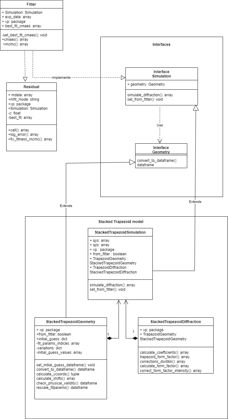
UML diagram of the design for CD-SAXS simulation application.

Interface Simulation:

An interface defines a contract that classes must follow, specifying a set of methods that implementing classes should have. In Python, I have chosen to use Protocol to achieve a similar effect. This is the base class for all simulation models. The functions and classes used in it should be implemented in all simulation models. This interface simplifies future model building by ensuring that simulation functions are not geometry-dependent.

Interface Geometry:

Similar to the Interface Simulation, this is the base class for all geometry models. This interface simplifies future model building by ensuring that geometry functions are not dependent on the specific simulation details.

Model:

In this UML diagram (fig-UML), we present the implementation of the stacked trapezoid model. Central to this model is the StackedTrapezoidSimulation class, which is a composite class integrating StackedTrapezoidGeometry and StackedTrapezoidDiffraction classes. The StackedTrapezoidGeometry class handles all geometrical calculations and stores the relevant information, while the StackedTrapezoidDiffraction class is responsible for all diffraction-related calculations.

These classes work together to simulate the physics and generate data that can be compared with experimental results. Throughout the project, additional models are being developed and will be discussed later. The stacked trapezoid model serves as a prototype, illustrating how other models will be implemented. Each model will adhere to the base interfaces Simulation and Geometry.

Relationships between components

This structure is designed to simulate and analyze diffraction patterns using a modular approach. At its core, the system comprises several key components: the Fitter, Residual, and interfaces for Simulation and Geometry, along with specific model implementations like the StackedTrapezoidSimulation. The Fitter class orchestrates the fitting process by using the cmaes function to estimate the best-fit parameters and the mcmc function to assess the uncertainty in the fit. It takes in a model and experimental data, utilizing the Residual class to compute the difference between the experimental data and the model simulated data. The Residual class leverages the model simulate_diffraction function to generate the diffraction pattern, which it then compares with the experimental data.

The model, meaning specific implementations of the interfaces, is designed to operate independently, allowing users to utilize a particular model for simulations without needing to engage with the fitting component. This autonomous functionality ensures that users can easily perform simulations solely with the model of their choice. This design choice enhances flexibility and usability, as it decouples the simulation process from the fitting procedures, making it more accessible for users who may only need to run simulations. The usefulness and implications of this design choice will be discussed shortly.

Creating a New Simulation Model

This section provides guidelines on how to develop a new simulation model that adheres to the established protocol. The protocol ensures compatibility between your simulation model and the fitter class, enabling seamless integration and functionality.

The protocol consists of a set of methods and properties that your Simulation and Geometry classes must implement. These classes form the core of your simulation model, handling the setup, execution, and data management for your simulations.

1. Geometry Class

   The Geometry class is responsible for defining the shape and structure of the system being simulated. It includes methods for converting simulation parameters into a structured format that can be used by the simulation engine.

   • convert_to_dataframe(fitparams): This method takes a list of fitting parameters (fitparams) and converts them into a pandas DataFrame. This DataFrame should be structured based on the initial guess values provided by the user.

     • Parameters: - fitparams (list): Array containing the parameters returned by the fitter.

     • Returns: - pandas.DataFrame: A DataFrame containing the parameters in a readable format.

2. Simulation Class

   The Simulation class orchestrates the simulation process. It uses the Geometry class to manage system structure and executes the core simulation logic.

   • geometry (property): This property returns an instance of the Geometry class, providing access to the geometric data of the system.

   • set_from_fitter(from_fitter): This method configures the simulation to recognize that the incoming data originates from a fitter object. It should also initialize necessary components, such as saving the initial guess to a DataFrame.

     • Parameters: - from_fitter (bool): Indicates whether the simulation is being driven by a fitter.

   • simulate_diffraction(fitparams=None, fit_mode=’cmaes’, best_fit=None): This method performs the actual simulation, generating the diffraction pattern or other relevant output based on the provided fitting parameters.

     • Parameters: - fitparams (list, optional): Parameters for the simulation, typically obtained from a fitter. - fit_mode (str, optional): Specifies the fitting method used (‘cmaes’ or ‘mcmc’). - best_fit (array-like, optional): The best-fitting parameters obtained from the fitter.

     • Raises: - NotImplementedError: If the method is not implemented in the derived class.

To develop a new model, you need to create classes that inherit from the Simulation and Geometry protocols and implement all required methods. Here’s how to approach this:

Look at the following tutorial to see how to implement a new model in the cdsaxs package.

• How to create a simulation Model for cdsaxs?
  • Create the Simulation Class
  • Define the Geometry Class
  • Separating the diffraction logic from the geometry

By following these guidelines, you can develop a new simulation model that integrates smoothly with the existing framework. The key is to ensure that all required methods and properties are properly implemented, allowing your model to function seamlessly within the larger simulation and fitting ecosystem. For getting concrete examples, you can refer to the existing models in the cdsaxs package, such as the Stacked Trapezoid and Strong Castle models.

Testing

Pytest is used for testing the codebase. The tests are located in the tests directory and are organized by module. When adding new features or modifying existing code, it is essential to write tests and check that the existing tests pass.

To run the tests, you need to install the testing dependencies. You can do this by running the following command:

(cdsaxs) $ pip install -r tests/requirements.txt

To run the tests, navigate to the root directory of the project and execute the following command:

(cdsaxs) $ pytest

Modifying and building the documentation

TO build the documentation, you need to install the dependencies which are listed in the docs/requirements.txt file. You can install them by running the following command:

(cdsaxs) $ pip install -r docs/requirements.txt

The documentation is built using Sphinx. To modify the documentation, navigate to the docs directory and edit the .rst files. Once you have made your changes, you can build the documentation by running the following command:

(cdsaxs) $ make html