Overview

Miniaturizing transistors, the building blocks of integrated circuits, presents significant challenges for the semiconductor industry. Precisely measuring these features during production is crucial for high-quality chips. Existing in-line metrology techniques, such as optical critical-dimension (OCD) scatterometry and critical-dimension scanning electron microscopy (CD-SEM), are nearing their limits. OCD struggles with the inherent limitations of light and shrinking features, while CD-SEM, despite providing valuable insights, is restricted by sampling area and resolution. To overcome these obstacles, the industry is exploring X-ray-based metrology. X-rays, with their shorter wavelengths, allow for more precise analysis and are sensitive to variations in composition, providing richer data.

CD-SAXS (Critical Dimension Small Angle X-ray Scattering) is a promising technique for nano-structure electronics. It uses a transmission geometry, sending the beam through the sample and the 750 micrometer-thick silicon wafer. The X-ray spot size varies between 10-1000 μm, enabling the measurement of small patterned areas. Studies have shown CD-SAXS’s effectiveness in characterizing the shape and spacing of nanometer-sized patterns.

Although several big companies are developing software for CD-SAXS, this technique is still in its infancy and there isn’t an open-source coherent package available for its data analysis. Thus, this cdsaxs package is aimed at providing simulation and fitting tools for CD-SAXS synchrotron data for researchers.

The collection of functions developed at CEA (French Alternative Energies and Atomic Energy Commission) by former PhD students and at Lawrence Berkeley National Laboratory and Brookhaven National Laboratory served as the foundation for this package.

Installation

Note

cdsaxs can currently be used on Python >=3.8, 3.9, 3.10, 3.11 and 3.12.

cdsaxs is available to install through pip:

# Within a venv:
(cdsaxs-venv) $ pip install cdsaxs

Creating an isolated Python environment

It is good practice to use a dedicated virtual environment for cdsaxs and its dependencies to avoid affecting other environments on your system. To achieve this you can use a virtualenv or a conda environment, according to preference.

Using virtualenv

You can use virtualenv or venv if you have a system-wide compatible Python installation. For Mac OS X, using conda is recommended.

To create a new virtualenv for cdsaxs, you can use the following command:

$ virtualenv -p python3 ~/cdsaxs-venv/

If multiple Python versions are installed, replace python3 with python3.9 or a later version.

Replace ~/cdsaxs-venv/ with any path where you would like to create the venv. You can then activate the virtualenv with

$ source ~/cdsaxs-venv/bin/activate

Afterwards, your shell prompt should be prefixed with (cdsaxs-venv) to indicate that the environment is active:

(cdsaxs-venv) $

Now the environment is ready to install cdsaxs using the pip command at the top of this page.

For more information about virtualenv, for example if you are using a shell without source, please refer to the virtualenv documentation. If you are often working with virtualenvs, using a convenience wrapper like virtualenvwrapper is recommended.

Using conda

If you are already using conda, or if you don’t have a system-wide compatible Python installation, you can create a conda environment for cdsaxs.

This section assumes that you have installed anaconda or miniconda and that your installation is working.

You can create a new conda environment to install cdsaxs with the following command:

$ conda create -n cdsaxs python=3.11

Activate the environment with the following command:

$ conda activate cdsaxs

Afterwards, your shell prompt should be prefixed with (cdsaxs) to indicate that the environment is active:

(cdsaxs) $

Now the environment is ready to install cdsaxs using the conda command at the top of this page.

For more information about conda, see their documentation about creating and managing environments .

Optional dependencies

The cdsaxs package is designed to work with cupy for GPU acceleration. To install the optional dependencies, use the following command:

(cdsaxs) $ pip install cdsaxs[gpu]

Background

Simulation models

Two models were considered in the development of this code. The first model focuses on the cross section of a line in a line-space pattern. In this model, the cross section of a line is represented by a stack of trapezoids, which collectively form the shape of the cross section. This model is known as the Stacked Trapezoid Model.

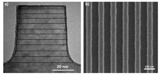
SEM image in a) is a cross-section of a line in SEM image in b). The black trapezoidal shapes in a) represent the modeling done for this simulation.

The second model introduces another concept known as the Strong Castle Model. This model builds upon the previous one by incorporating an additional nano-structure on top, resulting in an overlay. It provides a tool for representing the overlay between multiple structures.

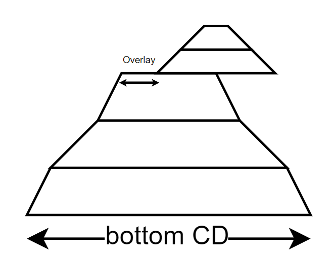
Strong castle model where top structure is not aligned thus we have an overlay.

To calculate the intensity profile of the scattering pattern, we perform a Fourier transformation on each trapezoid and then add them. The Fourier transformation of a trapezoid can be expressed using the following equation:

\[\begin{split}F\left(q_{x}, q_{z}\right)=\frac{1}{q_{x}}\left[-\frac{m_{1}}{t_{1}} e^{-i q_{x}\left(\frac{\omega_{0}}{2}\right)}\left(1-e^{-i h\left(\frac{q_{x}}{m_{1}}+q_{z}\right)}\right)\right. \\ +\frac{m_{2}}{t_{2}} e^{-i q_{x}\left(\frac{\omega_{0}}{2}\right)}\left(1-e^{\left.-i h\left(\frac{q_{x}}{m_{2}}+q_{z}\right)\right)}\right]\end{split}\]

where,

\[m_{1} = \tan\left(\beta_{1}\right)\]

\[m_{2} = \tan\left(\pi - \beta_{r}\right)\]

\[t_{1} = q_{x} + m_{1} q_{z}\]

\[t_{2} = q_{x} + m_{2} q_{z}\]

The \(\beta\)’s are the bottom side angles of the trapezoid. \(q_{x}\), \(q_{z}\) are the Fourier space coordinates, \(\omega_{0}\) is the width of the trapezoid, and \(h\) is the height of the trapezoid.

Fitting algorithm

The intensity map obtained from the synchrotron experiment looks like the following:

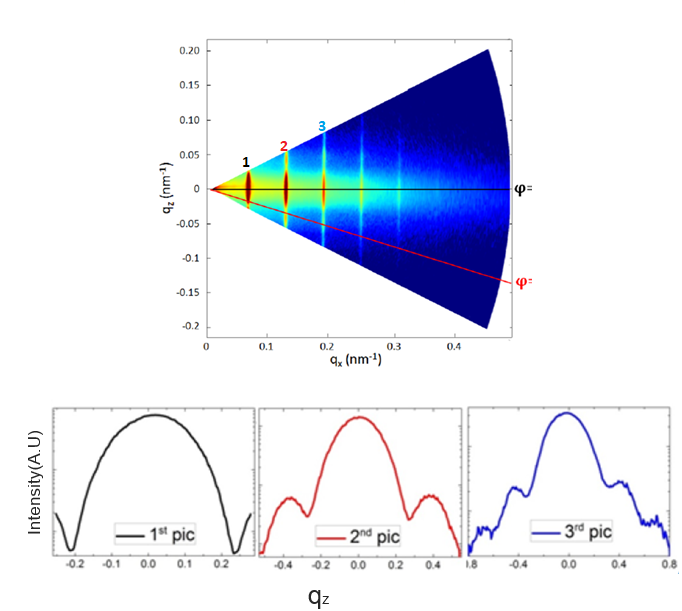
Intensity map and vertical cut of corresponding Bragg order

Vertical cuts along the different Bragg order are made to get the intensity profile shown below the intensity map. These profiles are the experimental data that we want to fit.

The objective of the fitting is to iterate over a high number of different line profiles (represented as various combinations of stacked trapezoids) and to converge towards the profile whose Fourier Transform will best match the experimental data. While the objective seems simple to describe, the problem is complex. Traditional optimization methods used for refinement often fall short when dealing with complex internal structures with numerous parameters, either being trapped in local minima or not converging toward the same solutions.

Another challenge arises from the possibility of “degenerate” solutions. These occur when multiple structural models can produce the same scattering data, making it difficult to pinpoint the true structure. This is a common issue in scattering analysis.

Therefore, the ideal scenario for CD-SAXS analysis involves an optimization algorithm that can consistently and rapidly converge on the best possible fit for the data. While some prior knowledge about the underlying structure can accelerate the process, such information is not always readily available. This highlights the need for more efficient algorithms that can handle complex structures even with limited prior knowledge.

Genetic and evolutionary algorithms have emerged as promising alternatives. These methods mimic biological evolution, with the model parameters acting as the “genetic code.” Starting with randomly generated parameters, these algorithms iteratively refine them through a “mixing strategy” over multiple generations until the optimal set is found. This approach excels at searching large parameter spaces with wide bounds, making it suitable for our purposes.

One algorithm is the Covariance Matrix Adaptation Evolution Strategy (CMAES). This method is particularly well-suited for high-dimensional optimization problems, making it ideal for complex nano-structure analysis. CMAES operates by maintaining a population of candidate solutions, with each iteration generating new candidates based on the previous generation’s performance. By adapting the covariance matrix of the candidate solutions, CMAES can efficiently explore the parameter space and converge on the optimal solution. The implementation of the deap library is used for this purpose.

For the CD-SAXS experiment, the algorithm starts with the experimental data collected. Then, a series of in-depth line profiles are generated through a set of parameters as described earlier. Afterwards, the calculated analytical Fourier transform is compared with the experimental data using a mean-absolute error log:

\[\Xi=\frac{1}{N_{q}-1}\sum_{q}|\log_{10}I_{Sim}(q)-\log_{10}I(q)|\]

where \(I_{\mathrm{Sim}}(\mathbf{q})\) is the simulated intensity and \(I(\mathbf{q})\) is the experimental intensity. \(\Xi\) is called the goodness of fit. The algorithm then tries to minimize \(\Xi\) by adjusting the parameters of the model.

We repeat this process until we are satisfied with the precision of the fit. The final set of parameters that gives the best fit and its fitness value is the output of the algorithm.

The CMAES algorithm provides a single best-fit solution for the nano-structure parameters. However, it is essential to understand the uncertainty associated with these parameters. This uncertainty relates to the different possible combinations of parameters that could result in a similar goodness of fit. For instance, slightly decreasing the height of one trapezoid and increasing the height of another can result in a similar goodness of fit. To address this, we can use the MCMC algorithm to explore and find all the sets of populations that can result in the same goodness of fit. The emcee library was very handy for this purpose.

Once all the populations of possible solutions are found, we can use them to obtain statistical information about the parameters. Notably, the uncertainty of the parameters using the confidence interval.