Synthetic Data - Compression Ratio 10x - Gaussian Noise
In this tutorial, we'll explore the process of reconstructing a phantom image using different methods and comparing the results.
Introduction
We demonstrates the use of different reconstruction methods on a phantom image of chromosomes. We'll use least-squares (LS), total variation (TV), and a neural network-based method called Noise2Ghost (N2G) to reconstruct the image [1]. We will impose a 10x compression ratio (10 times fewer measurements than reconstructed pixels), and add Gaussian noise to the measurements.
[1] M. Manni, D. Karpov, K. Joost Batenburg, S. Shwartz, and N. Vigano, "Noise2Ghost: self-supervised deep convolutional reconstruction for ghost imaging," Opt. Express, vol. 34, no. 13, p. 24787, Jun. 2026, doi: 10.1364/OE.596142.
Setup
First, let's import the necessary libraries and modules:
import matplotlib.pyplot as plt
import numpy as np
from autoden.models.config import NetworkParamsUNet
from corrct.param_tuning import get_lambda_range
from corrct.regularizers import Regularizer_TV2D
from corrct.processing.post import plot_frcs

from noise2ghost.reconstructions import RecParsCNN, fit_neural_cnn_reg_weight, fit_variational_reg_weight
from noise2ghost.testing import create_datasets
Creating the Dataset
We'll create a dataset using the create_datasets function. This function generates a phantom image of chromosomes and applies a sampling ratio of 10, photon density of 1e8, and readout noise standard deviation of 5.0.
info, volumes, data, _ = create_datasets(
    phantom_type="chromosomes",
    sampling_ratio=10,
    photon_density=1e8,
    reg_val_tv=None,
    readout_noise_std=5.0,
)
Note
We select the phantom type "chromosomes". Other options include: "dots", three flat dots (useful as an initial simple test case), "toy_xray", an X-ray image of a plastic toy, and "shepp-logan", which is the well-known Shepp-Logan phantom from the field of tomography. We set the compression ratio to 10x, by setting the value of the variable sampling_ratio.
Least-Squares Reconstruction
A LS reconstruction is provided by the synthetic data creation function. The LS minimizes the sum of the squared differences between the observed and predicted values.
gi_ls = np.squeeze(volumes["reconstruction_ls"])
Total Variation Reconstruction
Next, the TV regularized LS reconstruction is a method used to solve inverse problems where the solution is constrained by both the data fidelity term and a regularization term (i.e., the TV). In our case, the TV term promotes piece-wise constant regions in the reconstruction.
The forward model is defined by the equation: \(y = Wx\), where: \(y\) is the acquired data (measured buckets), \(W\) is the operator (stack of masks), and \(x\) is the sought solution.
The objective function for the TV regularized LS reconstruction is given by: $$ \hat{x} = \min_x { \frac{1}{2} || Wx - y ||_2^2 + \lambda || \nabla x ||_1 } $$ where \(\frac{1}{2} | Wx - y |_2^2\) is the data fidelity term, which ensures that the solution \(x\) is consistent with the acquired data \(y\), \(| \nabla x |_1\) is the TV regularization term, which promotes piecewise constant solutions and helps to remove noise and artifacts, and \(\lambda\) is the regularization weight that controls the trade-off between the data fidelity term and the regularization term.
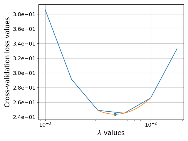
The value of \(\lambda\) is unknown and it depends on each specific acquisition. The strategy we use for selecting it is through the computation of a cross-validation loss over a hold-out set. More precisely, we set aside 10% of the acquired measurements, which are not used for reconstruction. We then sample a range of \(\lambda\) values, and compute one corresponding reconstruction each of those different values. We then compute the cross-validation loss over the hold-out set, and select the lambda value that minimizes it.
reg_vals_tv = get_lambda_range(1e-4, 1e-2)
best_reg_val_tv, volumes["reconstruction_tv"], _ = fit_variational_reg_weight(
    data["masks"], data["buckets"][0], reg=Regularizer_TV2D, lambda_range=reg_vals_tv, normalize=True
)
gi_tv = volumes["reconstruction_tv"]
Note
In the code above, the first line defines the range of the \(\lambda\) parameters to test.
Once the reconstruction is done, we can observe the cross-validation loss for all the tested \(\lambda\) parameters:
Noise2Ghost Reconstruction
Finally, we use the N2G algorithm to reconstruct the same data. We use a U-Net with 3 levels and 20 features, and organize our data into 6 splits and 4 different permutations. For the selection of the regularization value, we use the same strategy as for the TV reconstruction. For further details, we refer to the published article on N2G [1].
net_pars = NetworkParamsUNet(n_features=20, n_levels=3)
rec_pars_n2g = RecParsCNN(net_pars, num_splits=6, num_perms=4, epochs=1024 * 6)
reg_vals_n2g = get_lambda_range(5e-7, 5e-5)
best_reg_val_n2g, gi_n2g, losses, _ = fit_neural_cnn_reg_weight(
    data["masks"], data["buckets"][0], rec_pars=rec_pars_n2g, reg_vals=reg_vals_n2g
)
Results
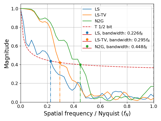
Let's first have a look at some performance metrics for the different reconstructions:
from skimage.metrics import mean_squared_error as mse
from skimage.metrics import peak_signal_noise_ratio as psnr
from skimage.metrics import structural_similarity as ssim

phantom = volumes["phantom"]
data_range = phantom.max() - phantom.min()

vols = [gi_ls, gi_tv, gi_n2g]
labs = ["LS", "LS-TV", "N2G"]

print("PSNR, range: [0, +inf), unit: [dB]")
for lab, vol in zip(labs, vols):
    print(f"- {lab:<8}: {psnr(phantom, vol, data_range=data_range):.4}")
print("SSIM, range: [0, 1]")
for lab, vol in zip(labs, vols):
    print(f"- {lab:<8}: {ssim(phantom, vol, data_range=data_range):.4}")
print("MSE, range: [0, +inf)")
for lab, vol in zip(labs, vols):
    print(f"- {lab:<8}: {mse(phantom, vol):.4}")

plot_frcs([(phantom, vol) for vol in vols], labs, snrt=0.4142)
Producing:
PSNR, range: [0, +inf), unit: [dB]
- LS      : 12.79
- LS-TV   : 22.47
- N2G     : 25.79
SSIM, range: [0, 1]
- LS      : 0.1237
- LS-TV   : 0.7038
- N2G     : 0.8036
MSE, range: [0, +inf)
- LS      : 0.03736
- LS-TV   : 0.004025
- N2G     : 0.001872
And then let's visualize the results of the different reconstruction methods:
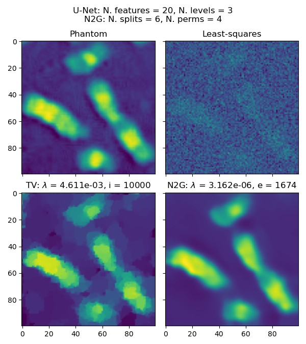
fig, ax = plt.subplots(2, 2, sharex=True, sharey=True, figsize=[6, 6.75])
fig.suptitle(
    f"U-Net: N. features = {net_pars.n_features}, N. levels = {net_pars.n_levels}\n"
    f"N2G: N. splits = {rec_pars_n2g.num_splits}, N. perms = {rec_pars_n2g.num_perms}"
)
vminmax = dict(vmin=phantom.min(), vmax=phantom.max())
ax[0, 0].imshow(phantom)
ax[0, 0].set_title("Phantom")
ax[0, 1].imshow(gi_ls, **vminmax)
ax[0, 1].set_title("Least-squares")
ax[1, 0].imshow(gi_tv, **vminmax)
ax[1, 0].set_title(f"TV: $\lambda$ = {best_reg_val_tv:.3e}, i = {rec_info_tv.best_residual_ind_val}")
ax[1, 1].imshow(gi_n2g, **vminmax)
ax[1, 1].set_title(f"N2G: $\lambda$ = {best_reg_val_n2g:.3e}, e = {np.argmin(losses['loss_tst'])}")
fig.tight_layout()