Tutorial for Strong castle model

This tutorial shows how to do simulations using strong castle model and how to fit the experimental data using this model.

from cdsaxs.fitter import Fitter
from cdsaxs.simulations.strong_castle import StrongCastleSimulation
import numpy as np

Simulation

Prepare the data

pitch = 100 #nm distance between two trapezoidal bars
qzs = np.linspace(-0.5, 0.5, 201)
qxs = 2 * np.pi / pitch * np.ones_like(qzs)

#Initial parameters
dwx = 0.1
dwz = 0.1
i0 = 10
bkg = 0.1
y1 = 0.
height = 10.
bot_cd = 40.
top_cd = 20.
swa = [90., 90.0, 90.0]
overlay = 10
#fixed parameters not be fitted
n1 = 2
n2 = 1

langle = np.deg2rad(np.asarray(swa))
rangle = np.deg2rad(np.asarray(swa))


overlay_params = {'heights': height,
            'langles': langle,
            'rangles': rangle,
            'y_start': y1,
            'bot_cd': bot_cd,
            'dwx': dwx,
            'dwz': dwz,
            'i0': i0,
            'bkg_cste': bkg,
            'overlay': overlay,
            'top_cd': top_cd,
            'n1': n1,
            'n2': n2,
            }

There are only 4 parameters that are different from the stacked trapezoid model, namely overlay, top_cd, n1 and `n2.

So the above parameters give us the following cross section:

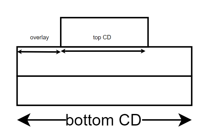
n1 and n2 correspond to the number of trapezoids in the bottom and top part of the model respectively.

Discussion about other parameters can be found in the stacked trapezoid model tutorial.

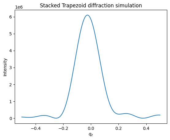
Now we will calculate the intensity exactly with strong castle model and plot the data.

Simulation1 = StrongCastleSimulation(qys=qxs, qzs=qzs)

intensity = Simulation1.simulate_diffraction(params=overlay_params)

#plot
import matplotlib.pyplot as plt
plt.plot(qzs, intensity)
plt.xlabel(r'$q_{z}$')
plt.ylabel('Intensity')
plt.title('Stacked Trapezoid diffraction simulation')

Text(0.5, 1.0, 'Stacked Trapezoid diffraction simulation')

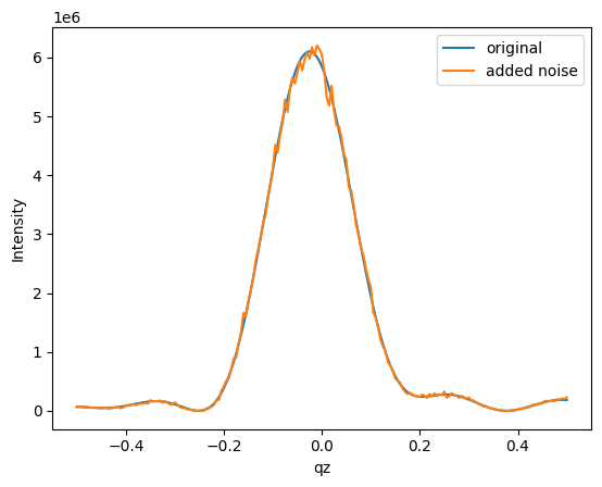
Fitting

We will do exactly the same steps as in the stacked trapezoid model tutorial. We will use the calculated intensities above as experimental and fit them with the strong castle model.

import matplotlib.pyplot as plt
intensity_noisy = intensity + np.sqrt(intensity) * np.random.normal(0, 50, intensity.shape)
plt.plot(qzs, intensity, label='original')
plt.plot(qzs, intensity_noisy, label='added noise')
plt.ylabel('Intensity')
plt.xlabel('qz')
plt.legend()


initial_params = {'heights': {'value': height, 'variation': 10E-3},
                    'langles': {'value': langle, 'variation': 10E-3},
                    'rangles': {'value': rangle, 'variation': 10E-3},
                    'y_start': {'value': y1, 'variation': 10E-3},
                    'bot_cd': {'value': bot_cd, 'variation': 10E-3},
                    'dwx': {'value': dwx, 'variation': 10E-5},
                    'dwz': {'value': dwz, 'variation': 10E-5},
                    'i0': {'value': i0, 'variation': 10E-5},
                    'bkg_cste': {'value': bkg, 'variation': 10E-5},
                    'overlay': {'value': overlay, 'variation': 10E-3},
                    'top_cd': {'value': top_cd, 'variation': 10E-3},
                    'n1': n1,
                    'n2': n2,
                    }

StrongCastle1 = StrongCastleSimulation(qys=qxs, qzs=qzs, initial_guess=initial_params)

Fitter1 = Fitter(Simulation=StrongCastle1, exp_data=intensity_noisy)

bestfit,fitness = Fitter1.cmaes(sigma=10, ngen=100, popsize=1000, mu=10, n_default=15, restarts=10, tolhistfun=10E-5, ftarget=10, restart_from_best=True, verbose=False)

print(bestfit)

    height1   langle1   langle2   langle3  rangle1   rangle2   rangle3  \
0  10.03779  1.651405  1.480153  1.592135  1.54748  1.708779  1.546373

    y_start     bot_cd       dwx       dwz         i0  bkg_cste   overlay  \
0  0.017236  40.000198  0.098872  0.100022  10.000337  0.099607  9.962454

      top_cd
0  19.999823

with np.errstate(divide='ignore', invalid='ignore'):
    stats = Fitter1.mcmc_bestfit_stats(N=15, sigma = 100., nsteps=200, nwalkers=1000)

print(stats)

15 parameters

100%|██████████| 200/200 [00:19<00:00, 10.10it/s]

               mean       std  count        min        max   lower_ci  \
height1   10.032762  0.154237  99987   8.643961  14.159510  10.031506
langle1    1.623662  0.050105  99987   0.190842   3.043659   1.623254
langle2    1.519561  0.066288  99987   0.058702   2.991455   1.519021
langle3    1.565897  0.066249  99987   0.156458   3.109113   1.565357
rangle1    1.489218  0.065244  99987   0.503257   2.847647   1.488687
rangle2    1.699659  0.067377  99987   0.002289   2.783351   1.699110
rangle3    1.529950  0.067966  99987   0.387656   3.065067   1.529396
y_start    0.457200  0.089482  99987   0.001071   1.319225   0.456471
bot_cd    39.984972  0.140185  99987  37.437256  41.138759  39.983830
dwx        0.098333  0.000941  99987   0.070365   0.127836   0.098326
dwz        0.100564  0.000768  99987   0.066336   0.108642   0.100558
i0        10.000036  0.000861  99987   9.958191  10.012195  10.000029
bkg_cste   0.099234  0.001000  99987   0.083602   0.113223   0.099225
overlay    9.806060  0.116891  99987   8.054958  13.368229   9.805108
top_cd    20.008583  0.087218  99987  18.643542  21.149993  20.007873

           upper_ci  uncertainity
height1   10.034019      0.001257
langle1    1.624070      0.000408
langle2    1.520101      0.000540
langle3    1.566436      0.000540
rangle1    1.489750      0.000532
rangle2    1.700208      0.000549
rangle3    1.530504      0.000554
y_start    0.457929      0.000729
bot_cd    39.986114      0.001142
dwx        0.098341      0.000008
dwz        0.100570      0.000006
i0        10.000043      0.000007
bkg_cste   0.099242      0.000008
overlay    9.807013      0.000952
top_cd    20.009294      0.000711