GUI description
Note
As of 2025, both GUIs (Tkinter and PySide) offer nearly identical features. Consequently, the descriptions below primarily refer to the Tkinter GUI. Any specificities of the PySide GUI will be detailed where applicable.
Files selection
The files selection is realized with the following widget:
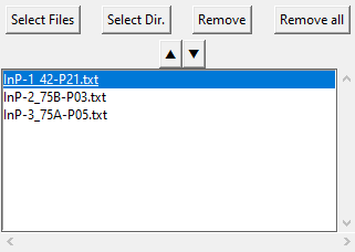
Select Files enables to load spectra (as ‘.txt’ files) selected individually or by block while Select Dir. loads all spectra that are contained in a selected directory.
2D-map: Once loaded in the GUI, if Fitspy detects that a ‘.txt’ file corresponds to a 2D-map input data file (via the tabulation t as first character), this one is expanded.
That is to say that each spectrum of the 2D-map appears individually in the files selection widget according to the 2D-map file basename and the (X) and (Y) spectrum coordinates in the grid as prefix:
{basename} X={X} Y={Y}
A 2D-map figure is also opened to facilitate both the spectrum selection and the interaction with the files selector widget. Additionally, it allows to see the fit parameters in 2D displaying.
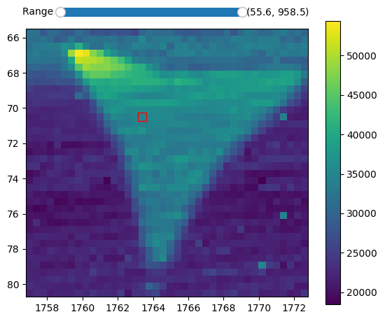
interactive 2D-map figure resulting from this fully defined ordered acquisition grid
Global actions (Tkinter)
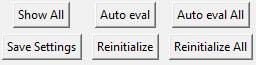
Show All enables a global display of all the spectra. When clicking on the canvas with the mouse, the nearest spectra are highlighted (up to a maximum of 10 spectra).
Auto eval and Auto eval All perform automatic evaluation of the baseline and peak positions and conduct fitting on the selected spectra or all the spectra (respectively).
Save settings enables the saving of user settings in a settings.json file located in the %HOMEUSER%/Fitspy directory (open this file to have a look on which and how settings are saved).
Reinitialize and Reinitialize All reinitialize the spectrum and all the spectra (resp.) to their original values.
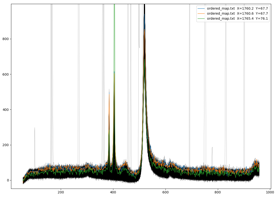
Example of the global display obtained with Show All
Overall settings
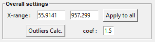
X-range allows the modification of the (x) support range associated with the current spectrum.
Apply to All applies the (x) support range defined in X-range to all the spectra.
Outliers Calc allows defining a line (called in Fitspy outliers_limit) from which values above are considered as outliers.
This line is defined as corresponding to the envelope of the spectra multiplied by the coef factor.
Consequently, the spectra loaded at the time of defining this line must be consistent with each other. (See here for more details).
Note
In the PySide GUI, the outliers envelop parameters settings and calculation are perform from the More settings panel
Baseline
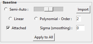
The current frame is activated and deactivated when clicking on it.
Semi-Auto allows a semi-automatic baseline determination based on the ARPLS (Asymmetrically Reweighted Penalized Least Squares) approach described here. The user only needs to adjust the smoothing coefficient with the slider beside that seems most likely to bring the baseline closest to the desired result.
Import enables the user to import their own baseline profiles. The imported file should contain 2 columns associated with the (x,y) coordinates of the baseline points.
Similar to spectrum profiles, the separators between the columns can be tabulation t, comma ,, semicolon ; or space .
Note that the first row is skipped, and the (x, y) rows can be unordered.
Auto can be used for the automatic determination of baseline points, considering the Min distance (minimum distance) between two consecutive points (in pixels).
Attached makes the baseline attached to either the raw spectrum profile or a smoothed one derived from Gaussian filtering applied to the raw spectrum profile, using Sigma as the standard deviation (in pixels).
Baseline profiles are defined either through Linear piecewise or Polynomial approximation, considering the specified Order.
It’s important to note that a ‘n’-order polynomial approximation requires at least ‘n+1’ points to be satisfied.
Normalization
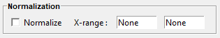
An optional spectra normalization is offered and relies on the two following strategies:
Maximum: when activated, each spectrum is normalized to 100 based on its maximum intensity on theX-rangespecified by the user. (None-None refers to no upper and lower x-range delimitation, that is to say all the support is considered).
Fitting
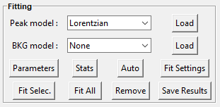
The current frame is activated and deactivated when clicking on it.
Auto can be used for the automatic determination of peaks, considering the selected Peak model.
For manual peaks positioning by the user, each Peak model (to be chosen between Gaussian, Lorentzian, Asymetric Gaussian, Asymetric Lorentzian, Pseudovoigt or as a user-defined model, see here) is applied when left-clicking in the figure. (A right-click in the figure removes the nearest peak).
Fit Selec. and Fit All perform the fitting based on the conditions defined in the Fit Settings widget for the Tkinter GUI and in the More Settings for the PySide GUI:
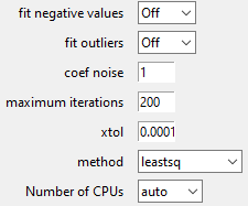
maximum iterations and xtol can be used to limit the number of iterations, saving CPU time processing consequently.
(An iteration corresponds to a gradient descent attached to all the fit parameters).
Spectrum fit success or failure (related to reaching a fit convergence criterion before reaching the maxmimum iterations) is displayed in green or orange (resp.) in the file selector widget.
It is worth noting that performing several successive fits on a spectrum may slightly change the fitted parameters.
Stats opens a frame that reports the statistics related to the fitting process.
The Parameters widget can be used to interact with each of the spectra (deleting or labeling peak models, redefining models, …).
By default, all parameters are considered as free but may be fixed during the fitting using the right-handed selection boxes.
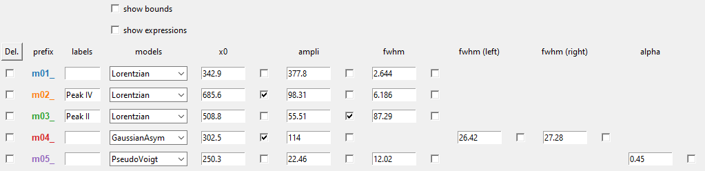
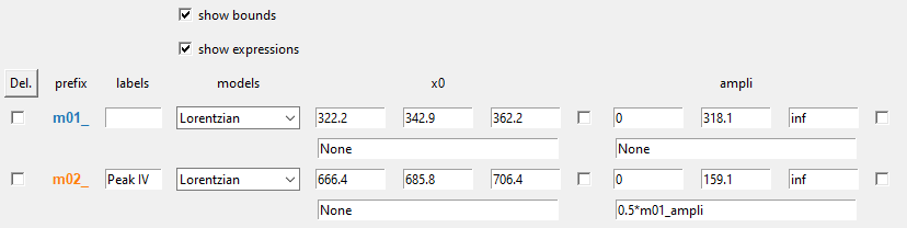
Bounds and fit constraints can be addressed by activating the dedicated selectors located at the top of the parameters widget.
Bounding consists in giving left and right parameters bounds.
Constraints relies on literal expressions that can be parameters-dependent, using the prefix defined in the 2nd column. The example below shows how to constrain the second fitted peak to be half the amplitude of the first one.
Save Results consists of saving the fitted parameters and related statistics in a folder predefined by the user, respectively in a .csv and a .txt file using the spectrum file basename (See here for more details).
Models (Tkinter GUI)
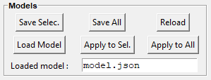
The Models frame is used to save and replay a full spectra processing as-is.
Save Selec. or Save All allows saving the spectra processing associated with the selected spectra in the files selection widget, or with all the spectra (resp.).
Reload replays exactly the spectra processing related to the imported .json.
This implies that all the files defined in the .json are reachable when reloading.
Load Model consists of reloading the first spectrum model (baseline and peaks definition, …) but not the spectrum file itself, related to the first model saved in the .json.
Apply to Sel. or Apply to All allows applying strictly (ie without considering the parameters defined in the GUI) the loaded model to the spectra selected in the files selection widget, or to all the spectra (resp.).
Models (PySide GUI)
TODO
Main Figure
The main Figure widget displays the loaded spectra and allows manipulation of baseline and peaks models with the mouse.
The standard navigation toolbar from Matplotlib allows panning, zooming and saving the current figure.
In the Tkinter GUI, the function associated with the  icon has been reconfigured to allow the figure rescaling on the current displayed spectrum.

Figure settings (at the top for the Tkinter GUI) and View Options (below the figure for the PySide GUI) allow personalizing plots displays, figure title, and axis labels (TO ADAPT for PySide).
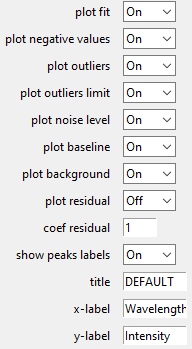
Save All (.png) (at the bottom) allows saving all the spectra figures in .png format. (Be cautious with 2D-maps as they can generate a large number of figures).
Note that to ease copy/paste, CTRL+C allows putting the current figure in the clipboard. (Only available on Windows).
2D-map Figures
The 2D-map Figure widgets allow easy selection of spectra and interaction with the cursor selection of the files selector widget.
By default, the full range of integrated spectra intensity is displayed with a range slider in the figure that allows specifying the summation bounds.
Once fitted, the parameters values can be visualized in the 2D-map figures.
All the maps displayed in the 2D-map Figure can be exported in a .csv file by clicking on the Export (.csv) button.
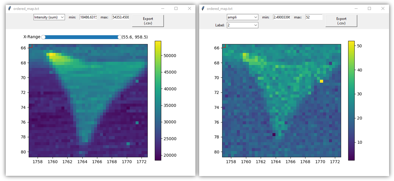
left: intensity field in a 2D-map figure (default mode). right: amplitude values associated to the 2nd peak (obtained after fitting).