Workflow

All the spectra fitting operations can be realized both through the GUI or by python scripts.

However, although python scripts can be very practical when working with repetitive actions (like batches in the case of parametric studies for instance), from a practical point of view, it is easier:

1/ to use the GUI to define a Fitspy model visually, then
2/ to apply it to new data sets.

GUI Mode

PySide GUI:

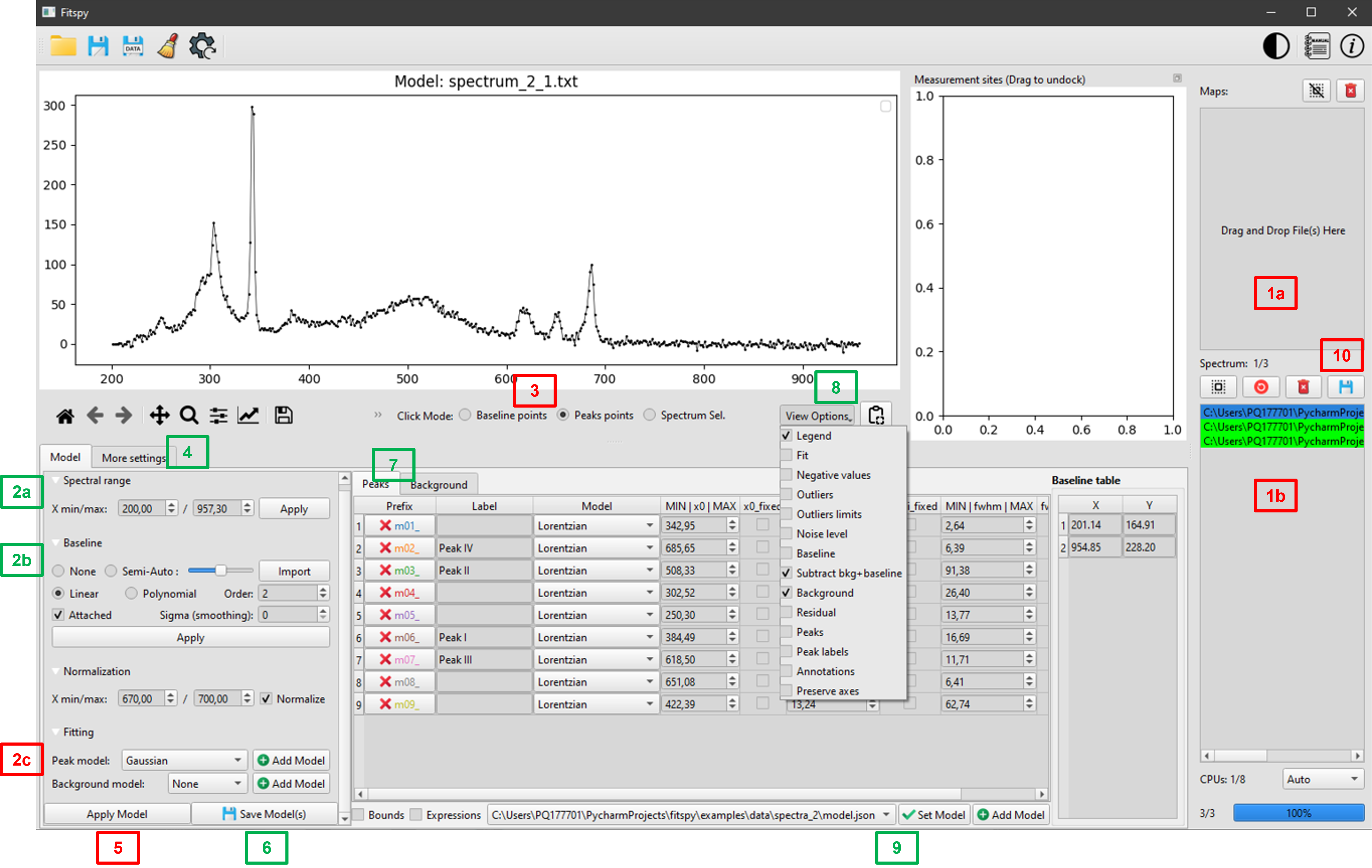
To create a `Fitspy` model:

(1) Select file(s) using drag an drop mode
(2a) Define the X-range
(2b) Select the baseline mode
(3) if Linear or Polynomial mode, click on the Baseline Points and select them on the main figure* (*)
(2c) Select a Peak model
(3) After clicking on Peaks points, Select them on the main figure (*)
(3) Add a background (BKG model) to be fitted
(4) Adjust extra-parameters
(5) Fit the spectrum/spectra selected in the files selector widget
(7) Use the peak and bkg tables to see the results and to set bounds and constraints for a new fitting
(6) Save the Model(s) in a `.json` file (to be replayed later)

(*) use left/right click on the figure to add/delete a baseline or a peak point

Once saved, a Fitspy model enables to recover a previous state (as-it, if all the spectra defined in the model can be loaded again) as follows:

(9) Add the `Fitspy` model (`.json` file)
(5) Fit the selected spectra
(10) Save Results (fitted parameters and statistics)

Or, after removing all spectra in the file selector widget (Remove All), the Fitspy model can be apply to another data set as follows:

(1) Select file(s) using drag an drop mode
(9) Add Model And select it from the Combobox
(15) Apply Model
(10) Save results (fitted parameters and statistics)

Tkinter GUI:

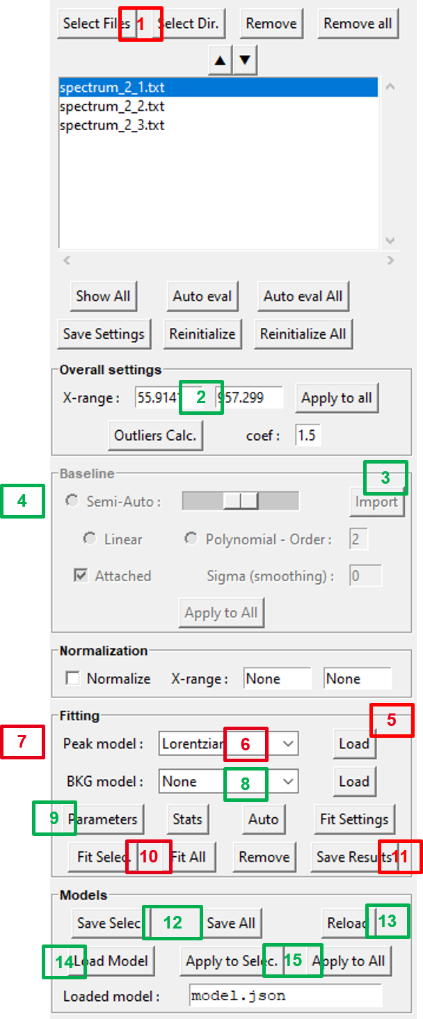
To create a `Fitspy` model:

(1) Select file(s) from Select Files or Select Dir
(2) Define the X-range
(3) Click on the Baseline panel to activate it (if not)
(4) Select baseline points on the main figure (*)
(5) Click on the Fitting panel to activate it (if not)
(6) Select a Peak model
(7) Select a peak point on the main figure (*)
(8) Add a background (BKG model) to be fitted
(9) Use Parameters to see the results and to set bounds and constraints for a new fitting
(12) Save Select or Save All the `Models` in a `.json` file (to be replayed later)

(*) use left/right click on the figure to add/delete a baseline or a peak point

Once saved, a Fitspy model enables to recover a previous state (as-it, if all the spectra defined in the model can be loaded again) as follows:

(13) Reload the `Fitspy` model (`.json` file)
(10) Fit Selec. or Fit All the spectra
(11) Save Results (fitted parameters and statistics)

Or, after removing all spectra in the file selector widget (Remove All), the Fitspy model can be apply to another data set as follows:

(1) Select file(s) from Select Files or Select Dir
(14) Load Model *(associated to the first spectra if several)
(15) Apply to Sel. or Apply to All
(11) Save Results (fitted parameters and statistics)

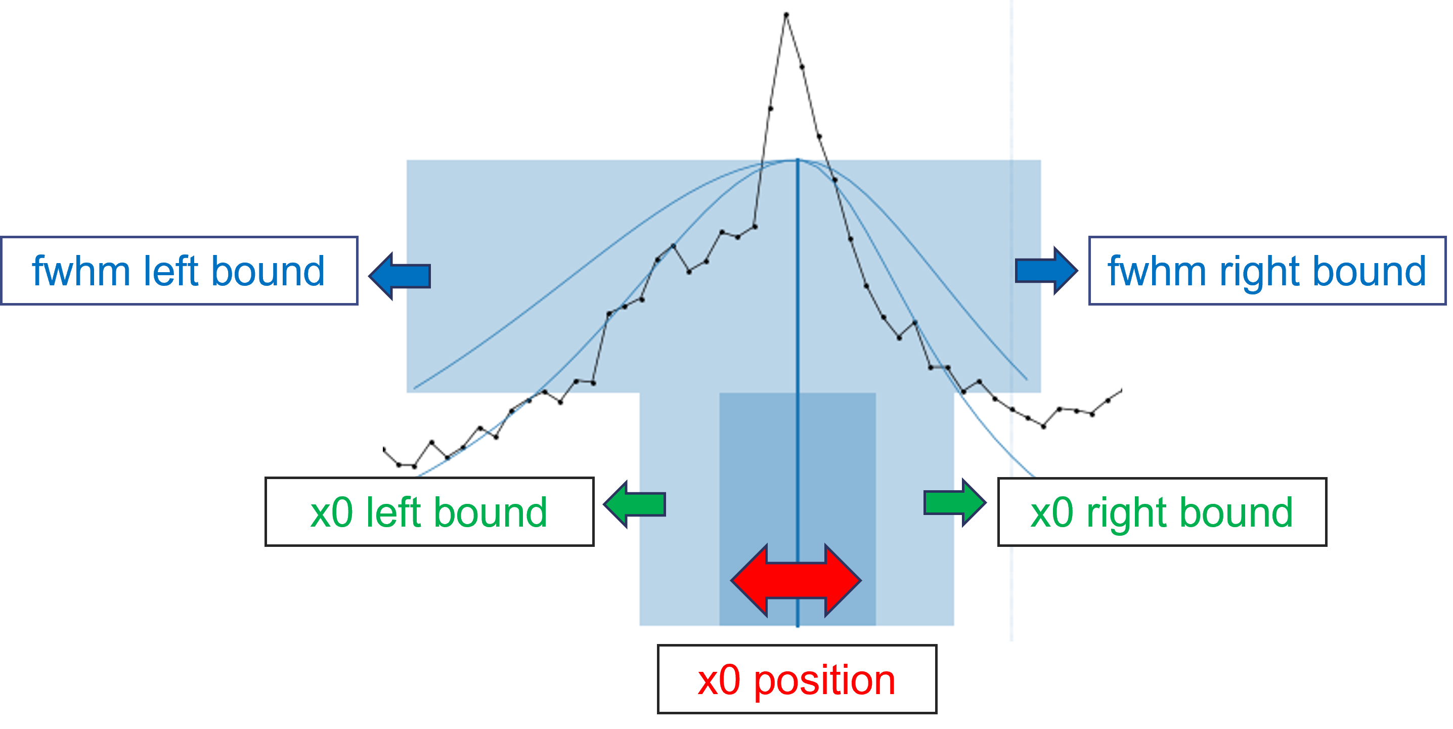
Interactive bounds:

Since version 2025.4, bounds can be adjusted interactively using the mouse.

When a new peak is added, model parameters are estimated based on the local profile of the spectrum.

The user can then move the entire set of bounding boxes by clicking and dragging the dark blue area, which updates the values of both x0 and ampli.

The bounds related to x0 and fwhm can be modified by dragging the left/right edges of the lower and upper bounding boxes, respectively.

Note that for symmetric models, the left and right fwhm bounds are synchronized, contrarily to asymmetric models that allow independent control of the left and right fwhm values.

Scripting Mode

Although it is more recommended to use the GUI to define a Fitspy model visually , here is a partial example of how to do it by script:

from fitspy.core.spectrum import Spectrum

spectrum = Spectrum()

# load a spectrum to create the model
spectrum.load_profile(fname=r"C:\Users\...\H-000.txt", xmin=150, xmax=650)

# baseline definition and subtract
spectrum.baseline.points = [[160, 600], [52, 28]] # (x, y) baseline points coordinates
spectrum.subtract_baseline()

# peak models creation (based on 2 peaks)
spectrum.add_peak_model('Lorentzian', x0=322)
spectrum.add_peak_model('Gaussian', x0=402)

# model saving
spectrum.save(fname_json=r"C:\Users\...\model.json")

Note

During the peak model creation, other parameters can be passed to add_peak_model() (see the API doc). Given the large number of parameters, only the main ones have been retained as arguments. Therefore, to have fine control over each parameter, you can use a dictionary as follows:

peaks_params = {1: {'name': 'Lorentzian',
                    'x0': {'value': 322, 'min': 300, 'max': 330},
                    'fwhm': {'value': 30, 'min': 22, 'max': 45}},

                2: {'name': 'Lorentzian',
                    'x0': {'value': 402, 'vary': False},
                    'ampli': {'expr': '0.5*m01_ampli'}},

                3: {'name': 'LorentzianAsym',
                    'x0': {'value': 445},
                    'fwhm_l': {'value': 30, 'min': 20, 'max': 47},
                    'fwhm_r': {'value': 20, 'min': 10, 'max': 25}}}

# create peaks with default values (name and x0 are the mandatory values)
for params in peaks_params.values():
    spectrum.add_peak_model(params['name'], params['x0']['value'])

# replace default values by the user's ones ('min', 'max', 'vary', 'expr')
for peak_model, params in zip(spectrum.peak_models, peaks_params.values()):
    [peak_model.set_param_hint(key, **vals) for key, vals in params.items() if key != 'name']

A full example is available here: ex_nogui_peak_models_parameters_setting.py

Once defined, a Fitspy model saved in a ‘.json’ file can be applied to a more consequent data set as follows:

from pathlib import Path
from fitspy.core.spectra import Spectra
from fitspy.core.spectrum import Spectrum


fnames = Path(r"C:\Users\...").glob('*.txt') # list of the spectra pathnames to handle
model = r"C:\Users\...\model.json" # model pathname to work with

# Spectra object creation
spectra = Spectra(fnames=fnames)

# Fitspy model loading and application
spectra.apply_model(model, ncpus=16)

# Calculated fitting parameters saving
spectra.save_results(dirname_results=r"C:\Users\...\results")