Background removal

Most of the stacks acquisition techniques can produce gray intensity variations due, for instance, to charging effects (on low conductive material) or to shadowing effects (when imaging an area deep inside the material).

The background removal process step aims at reducing these large-scale effects on the images, assuming a polynomial behaviour to be fitted and removed.

Note

This fit is realised through the resolution of a minimization problem with a least square algorithm that consists in 2D to:

Given a polynomial basis \([1, x, y, xy, x^2, ...]\), find the polynom coefficients \((a_0, a_1, a_2, a_3, a_4,...)\) such as:

\[\begin{aligned}{\underset {(x, y)\in \mathbb {RxR} \subset Img}{\operatorname {minimize} }}\quad &\|Img(x, y) - a_0.1 + a_1.x + a_2.y + a_3.xy + a_4.x^2 + ...\|^{2}\end{aligned}\]

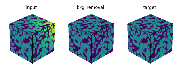
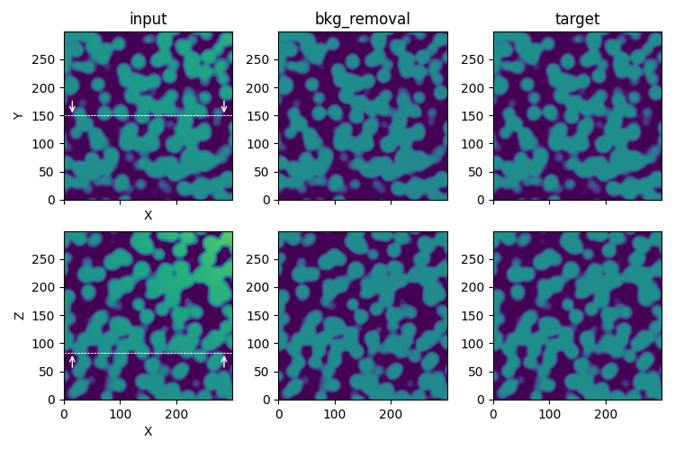
Illustration of the bkg_removal process step in the synthetic test case.

[bkg_removal]
dim = 3
#poly_basis = "1 + x*y*z"
orders = [1, 1, 1]
cross_terms = true
skip_factors = [5, 5, 5]
threshold_min = 5
#threshold_max = 10.
#weight_func = "HuberT"
#preserve_avg = true

The dim parameter defines the dimension of the problem to solve (2D or 3D):

• with dim = 3 a single resolution is performed (with a potentially high CPU cost) on the entire stack to determine the polynom coefficients. (The cost resolution can be significantly decreased using the skip_factor parameter, see below).

• with dim = 2 the resolution is performed slice by slice, leading to different polynom coefficients from one slice to another.

The 2D or 3D polynomial basis used to perform the fit can be defined in two ways:

• from poly_basis which defines the polynomial basis definition explicitly, term by term, from a literal expression

• from orders and cross_terms which define the basis implicitly in function to the order associated to each variable (x, y) in 2D or (x, y, z) in 3D.

Warning

Taking into account cross terms in the definition of the polynomial basis can prove crucial for achieving the desired fit. For instance, a background thought to be in the form of ‘xyz’ may actually have its minimum following a definition in ‘(x-a)(y-b)(z-c)’ in the reference basis used by the minimization procedure.

Since the images sizes and the number of frames could be big, the skip_factors parameter allows to significantly reduced the array to consider in the fitting processing. (Setting a skip_factors = [10, 10, 10] on a stack of size ~1000x1000x1000 seems to be a good compromise between accuracy, RAM occupancy and time execution).

When a skip factor is applied, the values taken into account are the ones corresponding to the indices positions. Using skip_averaging = true realizes a local averaging instead. (Note that no real benefit has been observed practically when activating this averaging).

Images may include regions that are not impacted (or slightly impacted) by the background effects like holes in a porous medium (characterized by very low values) or saturated pixels (characterized by very high values). For this reason, a mask to exclude values below threshold_min and above threshold_max can be defined to be applied during the fit processing.

The weight_func parameter (”HuberT”, “Hampel” or “None”) enables to specify (or not) a weight function used to determine and exclude outliers during the least squares problem resolution. See the RLM documentation for more details. (Default value is “HuberT”).

At last, the preserve_avg parameter enables to preserve the average between the input and the output data. The average preservation is suitable only when dim = 3. (Default value is False).

Plotting

The special plotting related to the bkg_removal process step generates images in the dedicated outputs folder that are named coefs.png, stats_X.png and stats_Y.png.

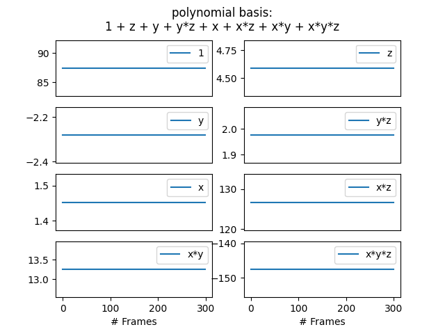
coefs.png gives the polynomial basis coefficients.

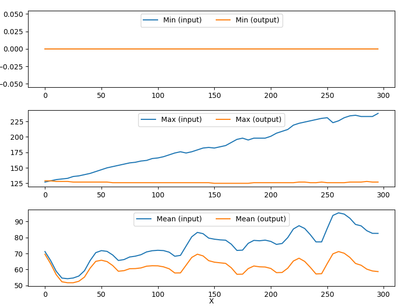
stats_X.png displays statistics along the ‘X’ axis.

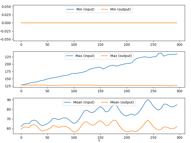
stats_Y.png displays statistics along the ‘Y’ axis.