Baselines and Background models

Two approaches are available in Fitspy to handle non-flattened profiles:

• the baseline approach

• the use of a background model during the spectra fitting

Baseline approach

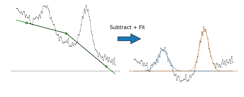
This approach involves either manually predefining points to establish the baseline profile that will be subtracted before fitting or a semi-automatic algorithm described hereafter.

Manual approach

From the baseline points, the profile all along the spectrum support is obtained by interpolation either from piecewise or polynomial approximations.

When setting a parameter named attached to True, the baseline points are attached to the corresponding spectrum intensity profile. This feature allows to adapt the baseline points to the spectrum notably when processing a dataset of spectra that have variations in intensity.

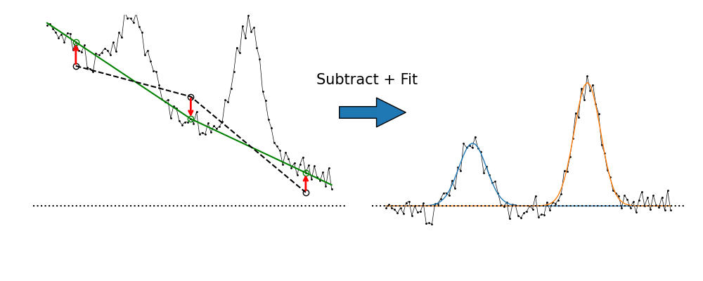
Note that to minimize the impact of noise in the baseline attached-points definition, a smoothing can be considered on the spectra intensities before linking. This smoothing is based on a gaussian filtering considering sigma (in pixel) as the standard deviation.

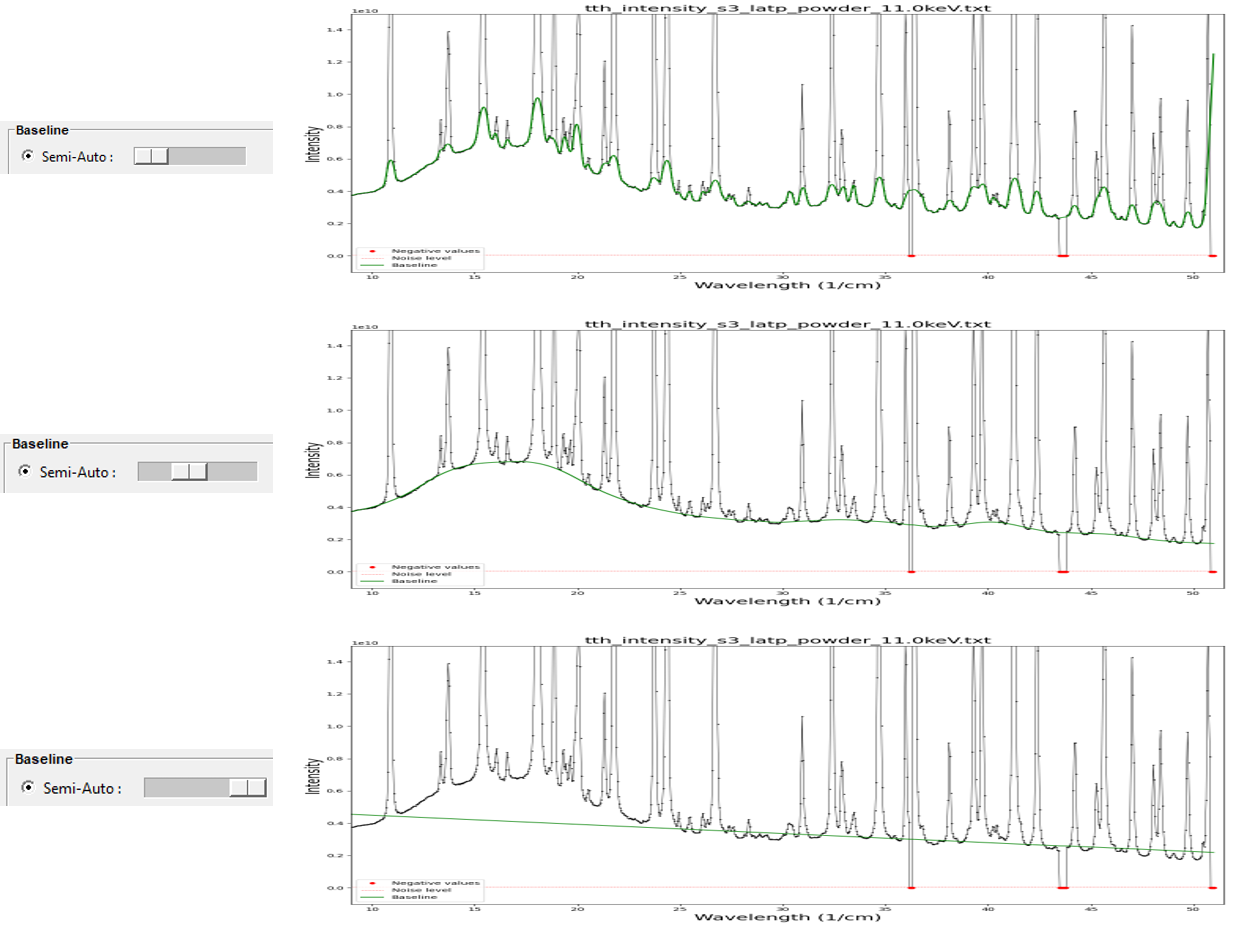
Semi-Automatic approach

From the 2024.5, a semi-automatic algorithm is availabel to evaluate the baseline. Based on the ARPLS (Asymmetrically Reweighted Penalized Least Squares) approach described here. The user only needs to visually adjust the smoothing coefficient that seems most likely to bring the baseline closest to the desired result.

Background model

The background model approach consists in selecting a BKG model that is taken into account with the peak models during the fit processing.

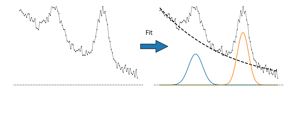
The available predefined BKG models are Constant, Linear, Parabolic, Exponential related to the lmfit standard models defined here.

User-defined background models

User-defined models can be defined through literal expressions in a ‘.txt’ file or from python scripts in a ‘.py’ file.

Example of two models defined by literal expressions:

Linear_1 = slope * x + intercept
Exponential_1 = ampli * exp(-coef * x)

Example of two models defined in python:

import numpy as np
from fitspy import BKG_MODELS


def linear(x, slope, constant):
    return slope * x + constant

def exponential(x, ampli, coef):
    return ampli * np.exp(-coef * x)

BKG_MODELS.update({"Linear_2": linear})
BKG_MODELS.update({"Exponential_2": exponential})

Through the GUI, the corresponding ‘.txt’ or ‘.py’ files can be loaded via the button Load located to the right of the BKG model combobox.

In python, the users models can be loaded by the related functions load_models_from_txt() and load_models_from_py(). (See example in ex_gui_users_defined_models.py )

For recurrent use, the user-defined models can be defined in files named bkg_models.txt or bkg_models.py to put in %HOMEUSER%/Fitspy.

The variable associated with the support must necessarily be used in expressions under the term x and the mathematical functions must be designated according to the terminology defined in the asteval package.

Note that in the examples given above, the resulting Linear_1, Linear_2 models yield identical results to those obtained from the predefined Linear model, when converged. The same for Exponential_1, Exponential_2 and Exponential.

Warning

Unlike predefined models, user-defined models do not have associated functions to determine their initial values for the fitting.

All the parameters are initialized to 1. This can lead to wrong convergence.

To prevent this, it is advisable to review the model parameters using appropriate multiplier coefficients.

Example: for a x-range in [0, 1000], the Exponential functions should be rather defined as ampli * exp(-coef * x / 1000)