Fitting

The fitting processing is performed using the methods provided by the lmfit package.

However, to facilitate the convergence of the fitting process, the signal can be pre-processed to subsequently distinguish between noise or outliers and ‘physical’ signal.

Noise level

After baseline subtraction, to avoid spending time in fitting peak models amidst noise, models in the ‘noisy regions’ are disabled.

A global noise level associated to each spectrum is first estimated (as the median of the absolute amplitudes of oscillating parts of the spectrum).

All peaks models located in areas below this noise level (multiplied by a user coefficient) are disabled and all the associated parameters (except x0) are set to 0.

Outliers

To determine outliers, a certain number of spectra of the same nature are required in order to be able to deduce numerically abnormal amplitude variations. This is well-suited particularly for 2D-map spectra.

First, a ‘normal spectra’ envelop is determined from the values of the 5th maximum intensity of all the spectra at any point (considering a null probability of having more than 5 outliers at the same point).

Outliers are then determined as points exceeding this envelope by a certain coefficient.

In the fit processing, outliers have a null weight associated with them (see below), and at the preceding baseline definition step, linear interpolations of the signal with respect to the points surrounding these outliers are performed.

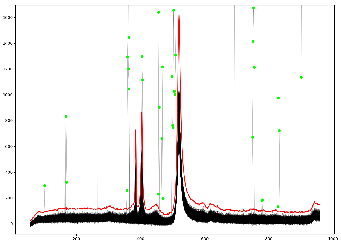
Illustration for a 2D-map spectra of the ‘normal spectra’ envelop (in red line) with coefficient 1.5, and resulting outliers (in green dots).

Fitting parameters

Fitting algorithm

In the GUI, the pre-selected fitting algorithms are Leastsq, Least_squares, Nelder-Mead, SLSQP which correspond in `lmfit` to the ‘leastsq’, ‘least_squares’, ‘nelder’ and ‘slsqp’ fitting algorithms (resp.).

In python script, all the allowed `lmfit` fitting algorithms can be used via the method argument passed to fit().

Convergence criterion

The convergence criterion is most often associated with a threshold to be reached on the calculated residual during the minimization procedure (gradient descent). Each fitting method used by `lmfit` has its own way of specifying this criterion. For Leastsq and Least_squares the xtol parameter can be pass to the fit function (see the scipy documentation for more details about this parameter). Otherwise, for the other fitting methods, in scripting mode, tolerance criteria can be passed through the fit_kws in the kwargs arguments of the fit() function (in a format compatible with the fit method).

This convergence criterion naturally has a significant impact on performance. (Refer to the section above).

Maximum number of iterations

This number, which corresponds to the maximum number of calls of the gradient descent process, is set by default to 200. It can be beneficial, when fitting numerous spectra, to decrease this value to save computation time, ensuring it does not significantly compromise the quality of the fits. Sometimes, just a few dozen iterations are indeed sufficient.

In the GUI, when the maximum number is reached without meeting the convergence criterion, the fit result is labeled as ‘non-converged’ and is displayed with an orange banner in the files selector widget. In case of convergence, the banner turns green.

Weighting

Similarly to noisy areas of outliers, the presence of negative values in the profiles to be fitted, resulting notably from baseline or background removal, can adversely affect the quality of results. To mitigate the impact of these negative values during the fit, a weight of ‘0’ can be assigned to them. This is achieved through the ‘fit negative values : Off’ option in the GUI or by the fit_negative parameter passed to fit().

(The same with fit_outliers for outliers and coef_noise to bypass regions defined mainly by noise).

Multi-threading

In the GUI, the default mode is ‘Number of CPU : auto’ which adapts automatically the number of CPU to the number of profiles to be processed and the CPU capability of the machine (by utilizing up to half of the available CPU resources).

Parameters values initialization

Also known as the Guess init step, the initial values assigned to the models parameters are crucial in the subsequent process of minimizing residuals through gradient descent. When poorly adapted to the profiles to be fitted, they can lead to inappropriate results (local minima), or even prevent the gradient descent. This is why the predefined models in Fitspy have their own methods for evaluating such initial values. The use of user-defined models without these methods and where all parameters are initialized to 1, can thus lead to bad convergence.

Note

It is possible that repeated actions of fits on a ‘converged profile’ may lead to small variations.

Constraints settings

Models parameters fixing

Each parameters can be set to free (default) or not during the fit processing. Fixing the parameters is achieved in the GUI by activating the boxes located to the right of each parameter.

Models parameters bounding

For each parameter, a range can be assigned for the fit processing. For the peaks models parameters, these ranges are defined at certain default values. In the GUI, these ranges can be adjusted through the Parameters widget by activating the show bounds box.

Models parameters coupling

Similarly, in the Parameters widget, constraints can be associated with each parameter, by activating the show expressions box and providing the constraints as explained here.

Performance

The performance varies depending on factors such as the number of spectra to handle, the number of points per spectrum, the number of peaks to fit, the xtol convergence criterion,… and, of course, the machine ‘s performance, including its multiprocessing capabilities.

Here is an example of the performance obtained from applying the Fitspy model.json (which includes the baseline removal and fitting 5 peak models per spectrum) to all 1520 spectra related to the example ex_gui_users_defined_models_2d_map.py.

Performance

Machine	Number of processors	xtol	CPU time (s)
PC Windows	8 (Intel(R) Core(TM) i5-10400H CPU @ 2.60GHz)	0.01	175
Windows server	36 (Intel(R) Xeon(R) Gold 6154 CPU @ 3.00GHz)	0.01	6
Windows server	36 (Intel(R) Xeon(R) Gold 6154 CPU @ 3.00GHz)	0.001	10
Windows server	36 (Intel(R) Xeon(R) Gold 6154 CPU @ 3.00GHz)	0.0001	18